Bayesian Logistic Regression

Formulation

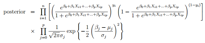
In this section, we start out by building our Bayesian logistic equation. We can define our posterior distribution as shown in the equation below. The likelihood is of the logistic regression form and the priors are normally distributed.

Features: diff_Pythag, diff_AdjOE, diff_AdjDE, location_Away, diff_RankAdjDE.

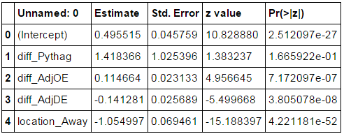
Next, we set the priors for our features listed above. We ran a logistic regression on all of the 2014 games and used the coefficients to inform us on how to set the priors for our Bayesian logistic regression. For our priors, we chose to use normals since the features are normally distributed. For the means, we use the estimate from the 2014 logistic regression. For the std, we chose 10 since the std error for the logistic regression are rather small.

Sampling Diagnostics

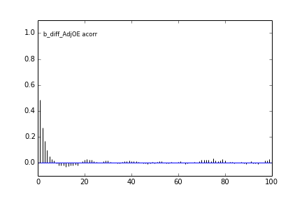
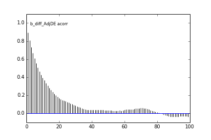
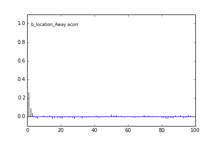
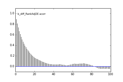
Autocorrelation

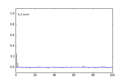
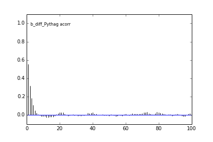
After setting up the features and priors, we can now run the MH sampling algorithm. We chose a burn-in rate of 5,000 points after observing the trace plots. Next, we also chose to thin and take 1 sample out of every 10 samples (this is detailed below). In summary, we will 105,000 points because we burn 5,000 points and take 1/10 every points. We also used the default proposal distribution to sample the target distribution with a standard normal.

Here are some autocorrelation diagnostic plots

Results from slice sampling are very similar.

Geweke Statistics

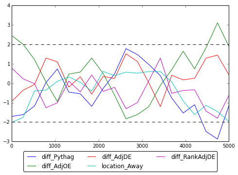
Lastly, we looked at whether our sampling method actually converged. To do this, we used the Geweke statistics. As seen below, most of the points are found to be between +/-2. Therefore, it is safe to conclude that the MH algorithm did indeed converge. For this section, we used pymc's geweke function.

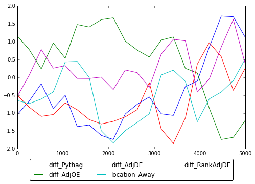
Here is the corresponding slice sampling Geweke Statistics plot.

Posterior Coefficient Means and Stds

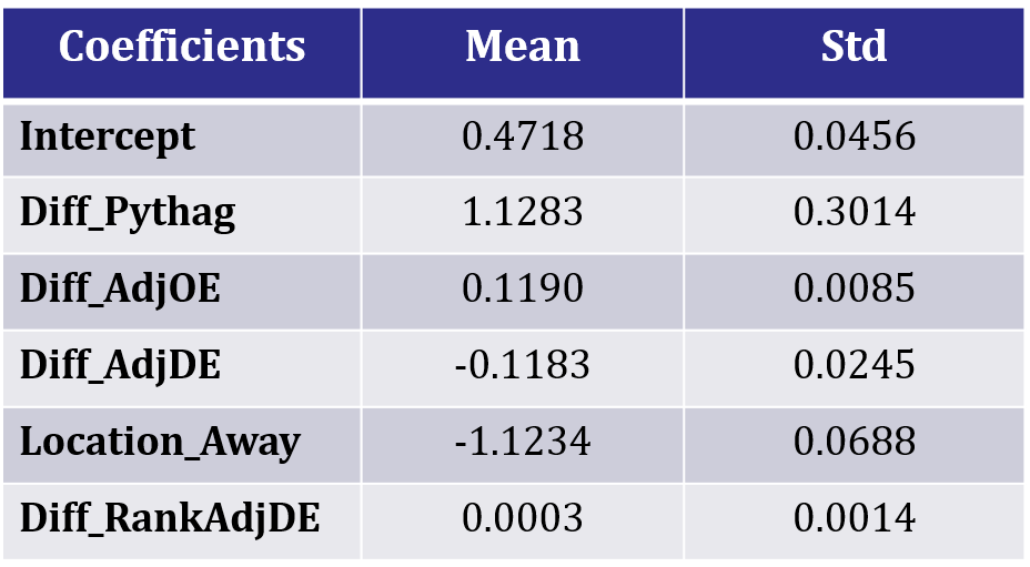
The posterior distribution results from slice sampling is very similar to those from MH. Therefore, we can be confident that we sampled the posterior distribution correctly. Using the two sets of results, we can use the coefficient samples for the 2015 NCAA simulations.

Predictions

Finally, before the long-awaited simulations, we can do a quick sanity check on our Bayesian logistic regression to see how well it actually performs on the actual 2015 NCAA tournament. First we predicted the outcomes for all 10,000 sets of coefficients that we sampled from the posterior distribution and calculated the average accuracy. Next, we also the accuracy from a model that uses the MAP coefficients.

From our results, we see that the 10,000 coefficients produced an average of 76.64% accuracy and the MAP coefficients produced an accuracy of 76.12% on the actual 2015 NCAA tournament! We are very satisfied with these results. Similarly, the slice sampler's coefficients produced 75.98% and 76.11% accuracy. Both sampling techniques resulted in very similar results and we are quite confident in our results going into the NCAA tournament simulation.